• ↑
  • Limiting Distributions

Central Limit Theorem

STA256

• Statistical Inference - STA258
• We have a population of any type or shape:
  • Normal Distribution
  • Exponential Distribution
  • Discrete Distribution
  • All of them will have $\mu ,\sigma$
• From the same population, if we take samples of size $n$.
  • $$\begin{array}{llll}\text{Sample 1}& \text{Sample 2}& \dots & \text{Sample 10 000}\\ \dots \}n& \dots \}n& & \dots \}n\\ \overline{X_1}& \overline{X_2}& & \overline{X_{10000}}\end{array}$$
  • Then we can create a distribution for our collection of $\overline{X}$'s.
  • Doesn't matter what the population is, the collection will be a bell curve.
  • $\overline{X}\stackrel{D}{\to }\mathrm{N}(\mu ,\frac{{\sigma }^2}{n})$
  • ${\mu }_{\overline{X}}=\mu$
  • ${\sigma }_{\overline{X}}^2=\frac{{\sigma }^2}{n}$
• So Central Limit Theorem tells us that:
  • $\overline{X}\stackrel{D}{\to }\mathrm{N}(\mu ,\frac{{\sigma }^2}{n})$
  • ${\displaystyle \frac{\overline{X}-\mu }{\frac{\sigma }{\sqrt{n}}}}\stackrel{D}{\to }\mathrm{N}(0,1)$
  • Even if you use Sample Variance, ${\displaystyle \frac{\overline{X}-\mu }{S}}$ also converges to a standard normal.
  • We can normalize it.
  • The transformation is $Z=\frac{x-\mu }{\sigma }$
    • Single observations
  • Working with samples of size $n$ we have a different transformation to provide the second normal distribution as $Z={\displaystyle \frac{\overline{X}-\mu }{\frac{\sigma }{\sqrt{n}}}}$
    • Sample means of size $n$
• As $n++$, the distribution of $\overline{X}$ becomes more normal. Sample size of $30$, is normally used to make it the theorem useful
• Example:
  • $\overline{X}$ is taken from a Gamma Distribution with $\alpha =2$ and $\beta =4$
  • Sample size $128$
  • $\overline{X}=X_1,X_2,\dots ,X_{128}$
  • $\overline{X}\sim \mathrm{\Gamma }(2,4)$
  • $\mu =\alpha \beta =(2)(4)=8$
  • ${\sigma }^2=\alpha {\beta }^2=(2)(4{)}^2=32$
  • $\sigma =\sqrt{32}=4\sqrt{2}$
  • Approximate $P(7<\overline{X}<9)$
    • $Z={\displaystyle \frac{\overline{X}-\mu }{\frac{\sigma }{\sqrt{n}}}}$
    • $Z={\displaystyle \frac{\overline{X}-8}{\frac{4\sqrt{2}}{\sqrt{128}}}}=2\overline{X}-16$
  • $P(7-\mu <\overline{X}-\mu <9-\mu )$
  • $P({\displaystyle \frac{7-\mu }{{\displaystyle \frac{\sigma }{\sqrt{n}}}}}<{\displaystyle \frac{\overline{X}-\mu }{{\displaystyle \frac{\sigma }{\sqrt{n}}}}}<{\displaystyle \frac{9-\mu }{{\displaystyle \frac{\sigma }{\sqrt{n}}}}})$
  • $P({\displaystyle \frac{7-\mu }{{\displaystyle \frac{\sigma }{\sqrt{n}}}}}<Z<{\displaystyle \frac{9-\mu }{{\displaystyle \frac{\sigma }{\sqrt{n}}}}})$
  • $P({\displaystyle \frac{7-8}{{\displaystyle \frac{4\sqrt{2}}{\sqrt{128}}}}}<Z<{\displaystyle \frac{9-8}{{\displaystyle \frac{4\sqrt{2}}{\sqrt{128}}}}})$
  • $P({\displaystyle \frac{7-8}{{\displaystyle \frac{4\sqrt{2}}{\sqrt{128}}}}}<Z<{\displaystyle \frac{9-8}{{\displaystyle \frac{4\sqrt{2}}{\sqrt{128}}}}})$
  • ${\displaystyle \frac{7-8}{{\displaystyle \frac{4\sqrt{2}}{\sqrt{128}}}}}=-2$
  • ${\displaystyle \frac{9-8}{\frac{4\sqrt{2}}{\sqrt{128}}}}=2$
  • $P(-2<Z<2)$
  • Go to the table, find $2.0$
    • $0.9772$
    • $1-0.9772=0.0228$
    • By symmetry
    • Bottom is $0.0228$
    • We have $0.9772-0.0228=0.9544$

STA260

• We just need our parent distribution to have a first and second moment.
• If we draw samples from any population (doesn't need to be normal or even continuous or discrete), which has a 1st, 2nd moments. Let the samples be of size $n$:
  • $\begin{array}{cccc}\text{Sample 1}:n,& \text{Sample 2}:n,& \dots ,& \text{Sample 10000}:n\\ {\overline{X}}_1& {\overline{X}}_2& \dots ,& {\overline{X}}_{10000}\end{array}$
  • We have here, a large collection of $\overline{X}$s.
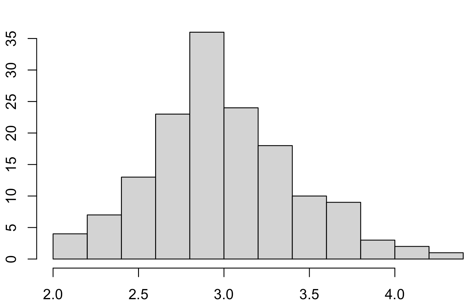
  • Then we can create a distribution for the collection of sample means (not the actual samples).
  • If you see an example histogram of the means. It resembles a normal distribution.
  • 
  • This is the sampling distribution of $\overline{X}$
  • So $\overline{X}\sim N({\mu }_{\overline{X}}=\mu ,{\sigma }_{\overline{X}}^2=\frac{{\sigma }^2}{n})$